Geostationary
GOES-R
The Geostationary Operational Environment Satellite R-Series is NOAA’s latest geostationary set of satellites. GOES-16, GOES-17, GOES-18, and GOES-19 are part of this series. The two instruments for terrestrial weather are the Advanced Baseline Imager (ABI) and the Geostationary Lightning Mapper (GLM).

Advanced Baseline Imager (ABI)
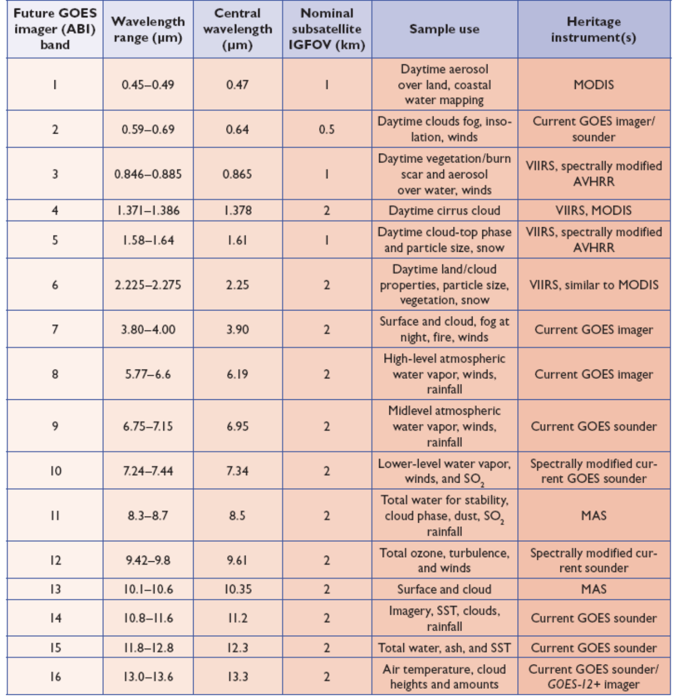
ABI consists of 16 channels and passively senses emitted and reflected radiation from visible, near-infrared, and longwave-infrared parts of the EM spectrum. The table summarizes some characteristics of the bands.
Quick Reference Guides
Here is a table with handy quick reference guides for the ABI Level 1b (L1b) bands.
Band Number |
Band Nickname |
Central Wavelength |
Quick Guide |
|---|---|---|---|
1 |
Blue band |
0.47 µm |
|
2 |
Red band |
0.64 µm |
|
3 |
Vegetation band |
0.86 µm |
|
4 |
Cirrus band |
1.38 µm |
|
5 |
Snow/Ice band |
1.61 µm |
|
6 |
Cloud Particle Size |
2.24 µm |
|
7 |
Shortwave infrared |
3.9 µm |
|
8 |
Upper-level water vapor |
6.19 µm |
|
9 |
Mid-level water vapor |
6.95 µm |
|
10 |
Low-level water vapor |
7.34 µm |
|
11 |
Infrared cloud-top phase |
8.6 µm |
|
12 |
Ozone band |
9.6 µm |
|
13 |
Infrared clean window |
10.35 µm |
|
14 |
Infrared window |
11.2 µm |
|
15 |
Infrared dirty window |
12.3 µm |
|
16 |
Carbon dioxide |
13.3 µm |
An important Level 2 (L2) product is the “Cloud and Moisture Imagery” (CMI), which is essentially the radiance from each L1b channel converted to reflectance or brightness temperature. Here is the quick guide for the CMI products. Here is a table with handy quick reference guides for the baseline ABI L2 products.
Baseline Level 2 Product |
Quick Guide |
|---|---|
Aerosol Detection Product (ADP) |
|
Aerosol Optical Depth (AOD) |
|
Derived Motion Wind vectors |
|
Derived Stability Indices |
|
Clear Sky Mask |
|
Cloud Phase |
|
Cloud-top Height |
|
Cloud-top Temperature |
|
Cloud-top Pressure |
|
Cloud-top Particle Size Distribution |
|
Cloud Optical Depth |
|
Volcanic Ash Detection |
|
IFR Probability |
|
Cloud Thickness |
|
Fire/Hotspot Characterization |
|
Land Surface Temperature |
|
Ice Concentration |
|
Ice Surface Temperature |
|
Ice Age/Thickness |
|
Ice Motion |
|
Snow Fraction |
Modes and sectors
ABI has multiple scan modes. In mode 4, or continuous full disk mode, the ABI produces a full disk (Western Hemisphere) image every five minutes. In mode 3, or flex mode, the ABI concurrently produces a full disk every 15 minutes, a CONUS image (resolution 3000 km by 5000 km) every five minutes, and two mesoscale domains (resolution 1000 km by 1000 km at the satellite sub-point) every 60 seconds or one sub-domain every 30 seconds. Mode 6, or 10-minute flex mode, which became the default operating mode for GOES-16 and GOES-17 in April 2019, provides a full disk image every 10 minutes, a CONUS (GOES-East) / PACUS (GOES-West) image every five minutes, and images from both mesoscale domains every 60 seconds (or one sub-domain every 30 seconds). All ABI bands have on-orbit calibration.
The pair of images below shows the increasing pixel area further away from nadir. The default east position is at 75 degrees west longitude; the default west position is at 137 degrees west longitude. Within the full-disk image, there is outlined the CONUS/PACUS and sample mesoscale sector domains.
Geostationary Lightning Mapper (GLM)
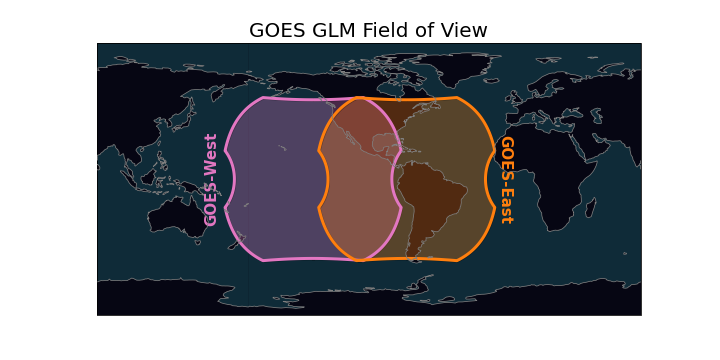
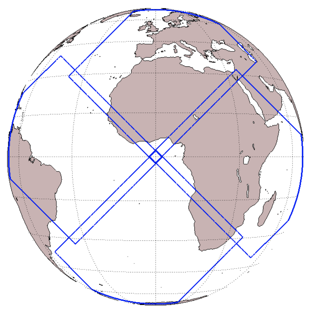
The GLM is the first-of-its-kind optical sensor from geostationary orbit. Its has a single near-infrared band at 777.4 nm. The instrument’s horizontal resolution ranges from about 8 km to 12 km. The image below shows the GLM’s field-of-view (FOV) [image credit: Brian Blaylock].
This set of quick guides provides a great overview of GLM events, groups, and flashes that the Lightning Cluster-Filter Algorithm (LCFA) creates, as well as information on higher-level gridded products, such as flash-extent density, average flash area, and total optical energy. The Level 2 files are produced every 20 seconds, with output from the LCFA. That is, the centroids of events, groups, and flashes. These point-based products are parallax-corrected using a “lightning ellipsoid,” which assumes a cloud height based on location and time of the year [FIXME: check time of year]. These files are available at all of the same sources wherer ABI is (see Data Access).
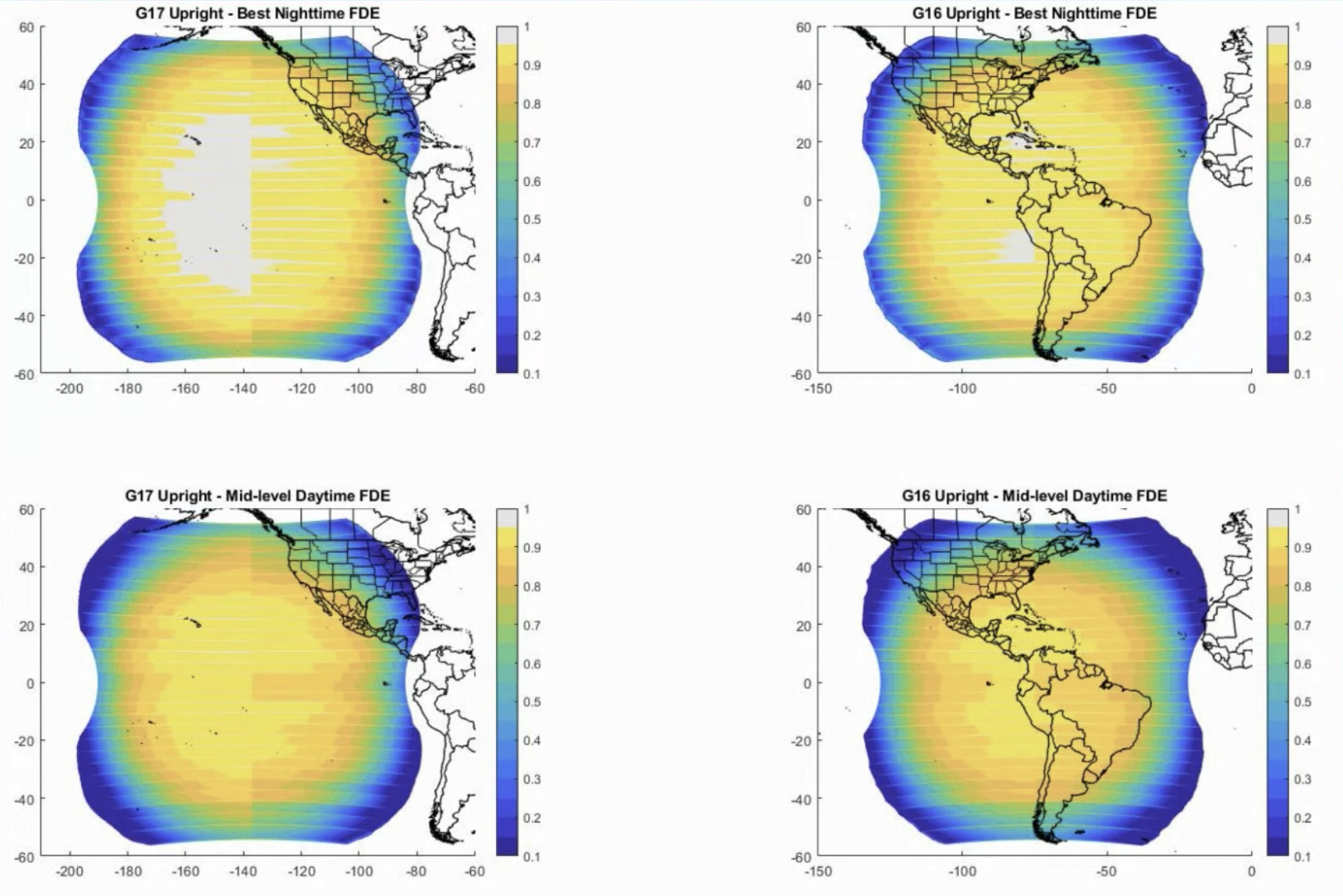
The flash detection efficiency of GLM varies as a function of viewing angle and solar illumination. The figure below summarizes this detection efficiency (source uknown). Users should be wary of using the data towards the limbs of the FOV.
Gridded GLM products
The best way to create the gridded products it to use glmtools. This page provides installation instructions and some examples of how to use the command-line utility, make_GLM_grids.py. From an operational perspective, the flash-extent density and minimum flash area (both available with glmtools) are the most used products. The flash-extent density provides the count of flashes that traverses a given pixel, whereas low minimum flash areas can indicate new storm updrafts. Note well: The gridded GLM products remove the parallax correction from the LCFA flashes. Thus, they match the un-corrected ABI data.
Data Viewing
There a number of excellent websites for GOES-16 imagery. Here are a few of my favorites:
Data Access
In lieu of a direct-broadcast antenna or LDM connection, the best way to obtain GOES-R data is probably through Amazon’s cloud (or Google, or Microsoft). GOES-2-Go is a handy tool to download data from AWS and create some quick-look images. Or you can use s3fs to directly access GOES-R data. NOAA’s CLASS is another option.
Using s3fs
On Linux command line, first pip install s3fs. Then using Python,
import s3fs
import xarray as xr
from datetime import datetime
import matplotlib.pyplot as plt
fs = s3fs.S3FileSystem(anon=True) #connect to s3 bucket!
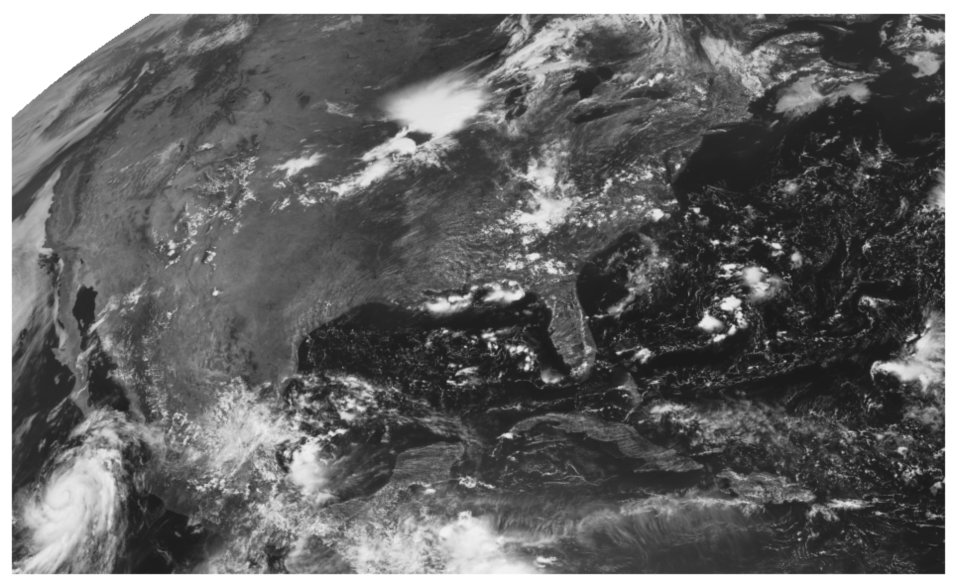
# Get the C02 CMI for 10 August 2020 18:01 UTC
abidt = datetime(2020,8,10,18,1)
file_location = fs.glob(abidt.strftime('s3://noaa-goes16/ABI-L2-CMIPC/%Y/%j/%H/*C02*_s%Y%j%H%M*.nc'))
file_ob = [fs.open(file) for file in file_location]
ds = xr.open_mfdataset(file_ob, combine='nested', concat_dim='time')
ch02 = ds['Rad'][0].data.compute()
# Make the image
# Note: I applied a square-root enhancement to make the land stick out more, but it is not necessary.
plt.imshow(np.sqrt(ch02), cmap="Greys_r")
plt.axis('off')
plt.show()
Using GOES-2-Go
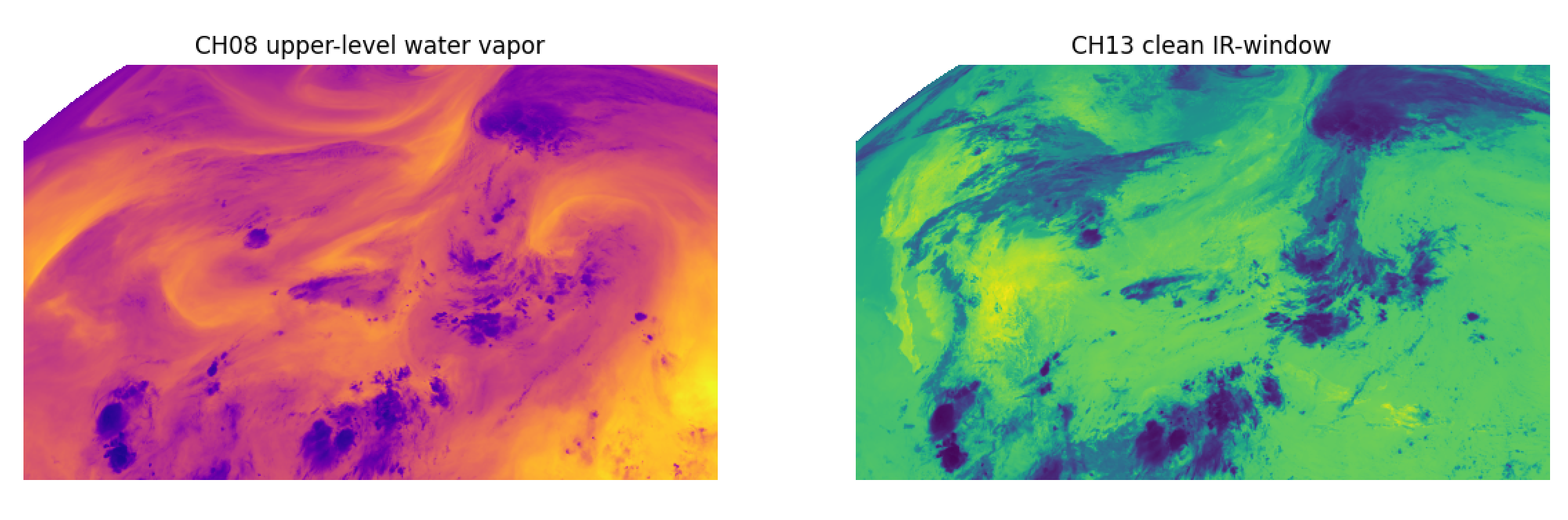
Here we use goes2go to get L1b data for two infrared bands, channels 08 and 13. We will convert them to brightness temperature ourselves.
from goes2go import GOES
import xarray as xr
import matplotlib.pyplot as plt

G = GOES(satellite=16, product="ABI-L1b-Rad", domain='C', bands=[8,13]) # leave out `bands` keyword if you want all channels.

# Download the latest available
ds = G.latest(download=False)  # `download=False` means reading from AWS to RAM directly.

# Convert to numpy.ndarray and convert to BT

# constants for ch08
planck_fk1 = ds['planck_fk1'].data[0]
planck_fk2 = ds['planck_fk2'].data[0]
planck_bc1 = ds['planck_bc1'].data[0]
planck_bc2 = ds['planck_bc2'].data[0]

ch08 = ds.Rad[0].data
ch08 = (planck_fk2 / (np.log((planck_fk1 / ch08) + 1)) - planck_bc1) / planck_bc2

# constants for ch13
planck_fk1 = ds['planck_fk1'].data[1]
planck_fk2 = ds['planck_fk2'].data[1]
planck_bc1 = ds['planck_bc1'].data[1]
planck_bc2 = ds['planck_bc2'].data[1]

ch13 = ds.Rad[1].data
ch13 = (planck_fk2 / (np.log((planck_fk1 / ch13) + 1)) - planck_bc1) / planck_bc2

fig,ax = plt.subplots(nrows=1, ncols=2, figsize=(12,5))
ax[0].imshow(ch08, cmap="plasma")
ax[0].axis('off')
ax[0].set_title('CH08 upper-level water vapor')
ax[1].imshow(ch13, cmap="viridis")
ax[1].axis('off')
ax[1].set_title('CH13 clean IR-window')
Notebook examples & exercises
Himawari
The Himawari geostationary satellites were launched and are managed by the Japanese Meteorological Agency (JMA). The main instrument, AHI, covers east Asia, the west Pacific, and Australia.
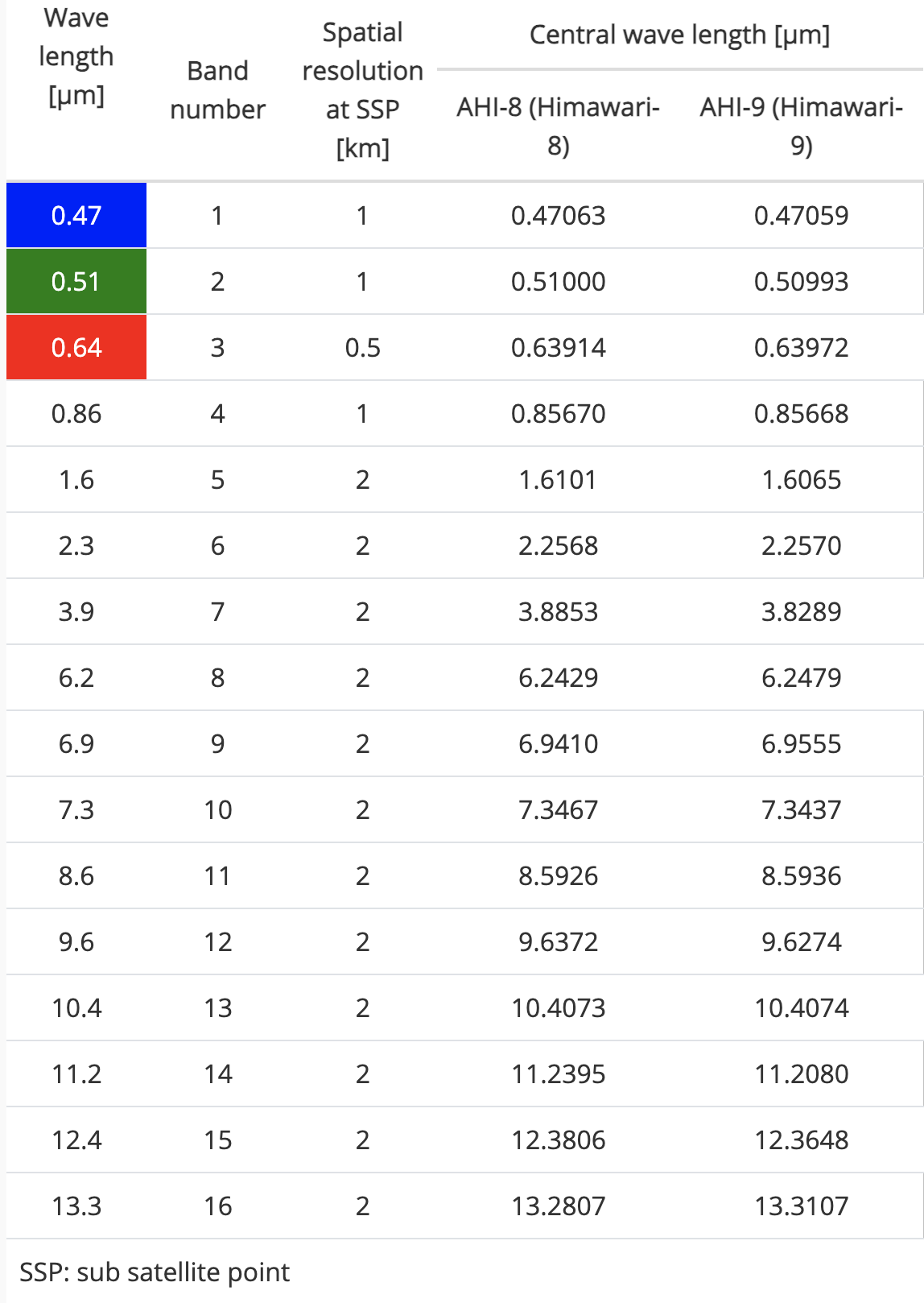
Advanced Himawari Imager (AHI)
The AHI was designed based off of ABI (Himawari-8 actually had the first ABI-generation imager launched into space!), but with a few differences:
AHI has a green visible band (0.51 µm), but ABI does not.
ABI has a cirrus band (1.38 µm), but AHI does not.
The 0.64-µm band is “B03” on AHI, whereas it is “C02” on ABI.
The resolution of B05 (1.6 µm) on AHI is 2 km, whereas the resolution of C05 (1.6 µm) on AHI is 1 km
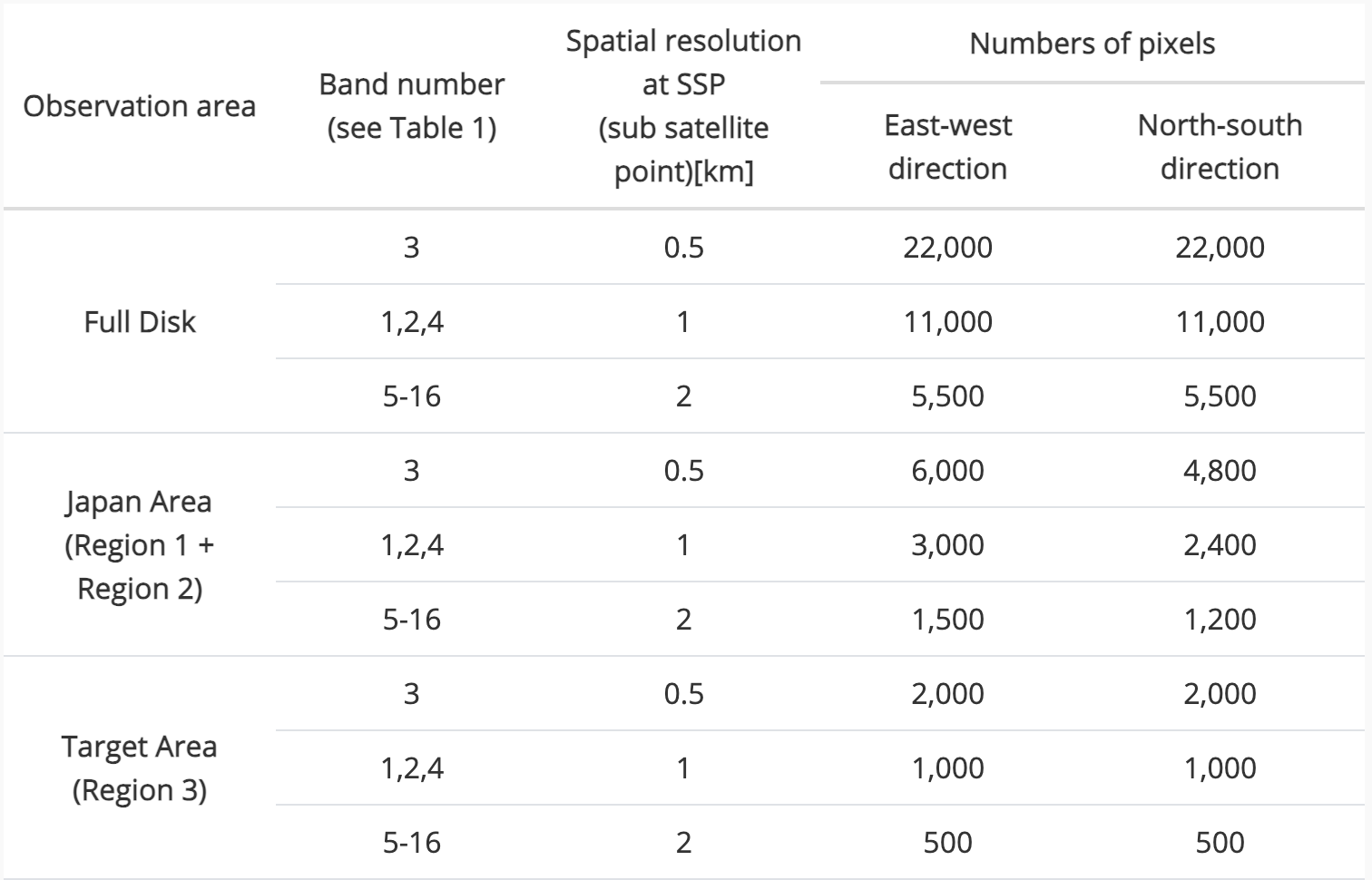
The table below summarizes the 16 AHI bands.
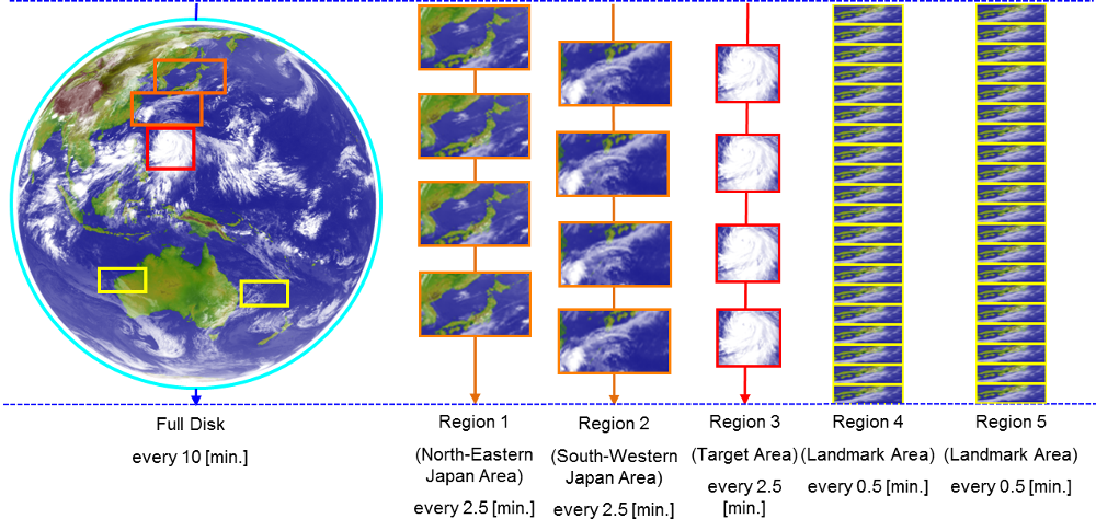
Sectors
AHI has the following sectors:
Full disk (every 10 minutes)
Japan (every 2.5 minutes, divided into two sub-sectors)
Target region (every 2.5 minutes)
The image and table below show some characteristics of the sectors. The “Target region” is analogous to ABI’s mesoscale sector, but it updates every 2.5 minutes instead of every 1 minute.
Data Viewing
Here are a few nice webpages to view real-time imagery.
Data Access
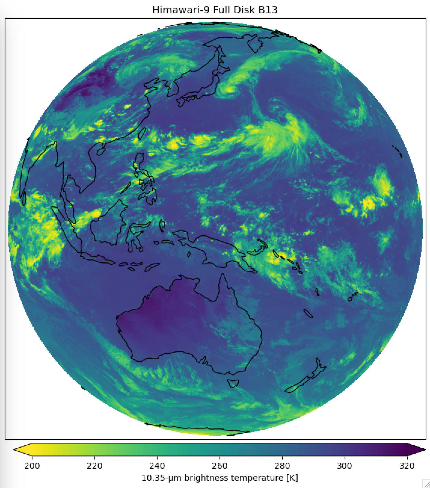
Himawari data can be accessed via NOAA’s Open Data Dissemination Program (NODD). See here for AWS data for Himawari-9. The script below will download the data and use satpy to read the remote files and process the data for visualization. Satpy is a very powerful tool for satellite I/O and processing. It can handle files from ABI, AHI, FCI, ATMS, VIIRS, IASI, and other instruments.
import matplotlib.pyplot as plt
from datetime import datetime
import os
import satpy

dt = datetime(2024,8,10,6,20)

# Read remote files on NODD/AWS
# Note the reader is 'ahi_hsd' for Himawari
storage_options = {'anon': True}
filenames = [dt.strftime('s3://noaa-himawari9/AHI-L1b-FLDK/%Y/%m/%d/%H%M/HS_H09_%Y%m%d_%H%M_B13_FLDK_R*_S*.DAT.bz2')]
scene = satpy.Scene(reader='ahi_hsd', filenames=filenames, reader_kwargs={'storage_options': storage_options})

# "Load" the band(s) we want to work with. Can do multiple bands, if the `filenames` included multiple bands.
scene.load(["B13"])

# Get the CRS, embedded in the Scene
crs = scene["B13"].attrs["area"].to_cartopy_crs()

# Set up the figure
fig = plt.figure(figsize=(7, 7))
ax = fig.add_axes([0, 0, 1, 1], projection=crs)
ax.coastlines()

# Get the data and use imshow to visualize
ir_data = scene["B13"].compute().data
img = ax.imshow(
    ir_data,
    transform=crs,
    extent=crs.bounds,
    vmin=200,
    vmax=320,
    cmap=plt.get_cmap("viridis_r"),
)
plt.title('Himawari-9 Full Disk B13')

cbar_axes = [0.02, -0.04, 0.98, 0.03] # left bottom width height

cbaxes2 = fig.add_axes(cbar_axes)
cbar2 = plt.colorbar(
   img,
    orientation="horizontal",
    extend="both",
    ax=ax,
    cax=cbaxes2,
)
cbar2.set_label('10.35-µm brightness temperature [K]', fontsize=10)

plt.savefig('h9_b13_FD.png',bbox_inches='tight')
Meteosat Third Generation (MTG)
Flexible Combined Imager (FCI)
The FCI has 16 spectral ranges covering visible to infrared wavelengths. The table below shows the FCI spectral channel spectral and spatial resolutions. The spectral channels VIS 0.6, NIR 2.2, IR 3.8 and IR 10.5 are delivered both in Normal Resolution (NR) and High Resolution (HR) spatial sampling configurations.
Spectral Channel |
Central Wavelength |
Sepctral Width |
Nadir resolution |
|---|---|---|---|
VIS 0.4 |
0.444 µm |
0.06 µm |
1.0 km |
VIS 0.5 |
0.510 µm |
0.04 µm |
1.0 km |
VIS 0.6 |
0.640 µm |
0.05 µm |
1.0 km; 0.5 km (HR) |
VIS 0.8 |
0.865 µm |
0.05 µm |
1.0 km |
VIS 0.9 |
0.914 µm |
0.02 µm |
1.0 km |
NIR 1.3 |
1.380 µm |
0.03 µm |
1.0 km |
NIR 1.6 |
1.610 µm |
0.05 µm |
1.0 km |
NIR 2.2 |
2.250 µm |
0.05 µm |
1.0 km; 0.5 km (HR) |
IR 3.8 |
3.800 µm |
0.40 µm |
2.0 km; 1.0 km (HR) |
WV 6.3 |
6.300 µm |
1.00 µm |
2.0 km |
WV 7.3 |
7.350 µm |
0.50 µm |
2.0 km |
IR 8.7 |
8.700 µm |
0.40 µm |
2.0 km |
IR 9.7 |
9.660 µm |
0.30 µm |
2.0 km |
IR 10.5 |
10.50 µm |
0.70 µm |
2.0 km; 1.0 km (HR) |
IR 12.3 |
12.30 µm |
0.50 µm |
2.0 km |
IR 13.3 |
13.30 µm |
0.60 µm |
2.0 km |
The images below show the approximate pixel area in km^2, assuming 1-km spatial resolution at nadir. You can see how pixel area increases rapidly once you hit 4-5 km^2. Figures are courtesy of EUMETSAT. The red dots in the second figure are cities, from south to north: Madrid, Prague, Stockholm, and Helsinki.
Scan Modes
FCI has two scanning modes:
Full Disc Scanning Service (FDSS) — provides observations in all of the 16 spectral channels (NR) and 4 spectral channels at high resolution (HR) (see Table 1) over the full disc visible from the geostationary 0° longitude position. The update time is 10 minutes.
Rapid Scanning Service (RSS) — provides samples in all of the 16 spectral channels (NR) and 4 spectral channels at high resolution (HR) (see Table 1) over the quarter of the disc, LAC4_4 (i.e., Europe and far Northern Africa). The update time is 2.5 minutes.
The nominal operational mode is based on two imager satellites. In the full operational constellation, one MTG-I satellite performs the full Earth-disc scanning in a 10-minute repeat cycle, the second covers the northern quarter of the full disc, over Europe in 2.5 minutes. See the FCI data guide for more details.
File Format
The file format is rather long for FCI data. Most users will only be interested in the Level 1c (Level 1b science data rectified to a reference grid) or Level 2 (Level 1b or Level 1c science data converted to geophysical values). Fortunately, the data are in netCDF4.
The most important parts are the start_time and end_time. The yyyyMMddhhmmss refers to the processing time of the file.
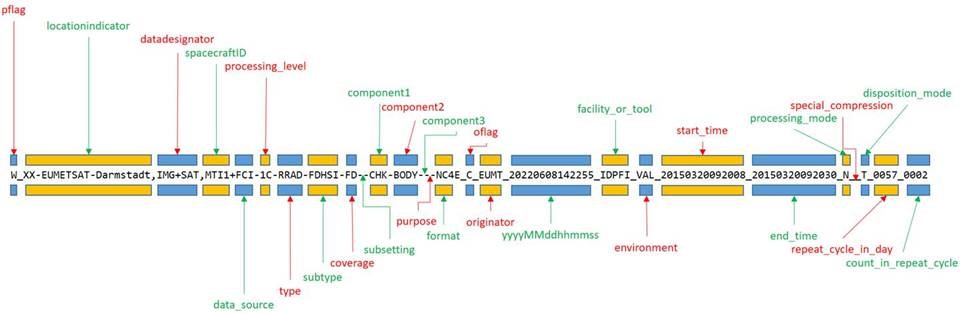
All of the FCI channels are in the same netCDF (unlike ABI). Each channel is in up to two netCDF groups: FDHSI (Full Disk High Spectral Resolution Imagery), and HRFI (High Spatial Resolution Fast Imagery).
Lightning Imager (LI)
The main benefits of geostationary lightning observations are that they provide homogeneous and contiuous information on lightning location and frequency, at low latency. Like the GOES-R GLM, MTG’s Lightning Imager (LI) has a single band at 777.4 nm, and can detect optical emissions from both in-cloud and cloud-to-ground lightning. Lightning is not recognized by its bright radiance alone, but by its transient short pulse character, possibly also against a bright background. A variable adapting threshold has to be used for each pixel which takes into account the change in the background radiance.
LI has a nadir resolution of 4.5 km. Like GLM, it also organizes observations into events, groups, and flashes, based on an algorithm with time and space thresholds. See the example below of the Level-2 processing sequence from LI (courtesy of EUMETSAT).
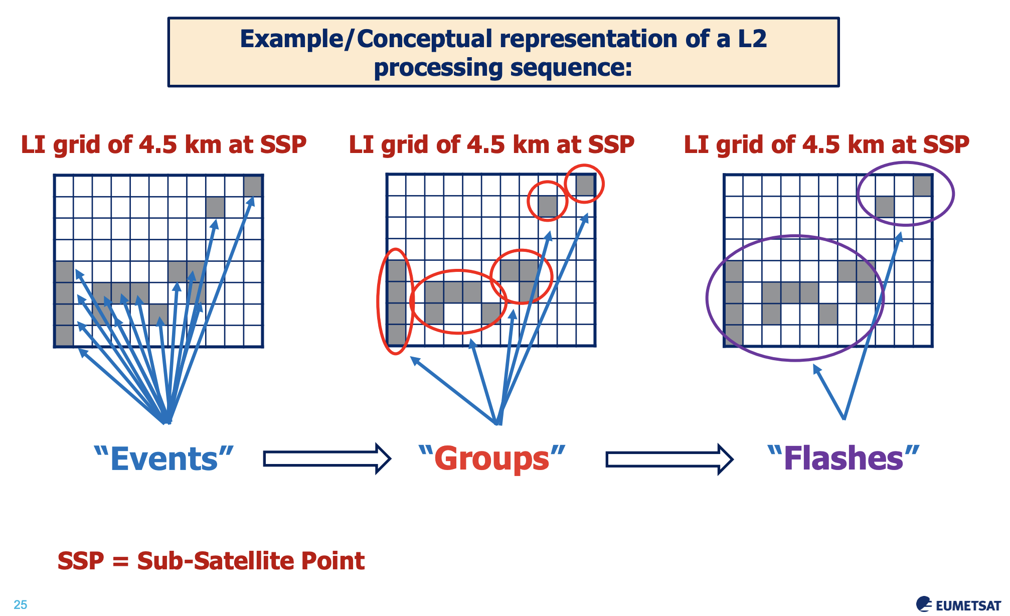
The LI domain consists of an area covered by four identical detectors with a small overlap. However, users of the Level-2 products will not “see” the detector structure. The pixel area for LI degrades quickly 50-70 km^2 (figures courtesy of EUMETSAT).
Data Types
There are 6 products for LI:
Collection |
ID |
|---|---|
LI Lightning Events Filtered - MTG |
|
LI Lightning Groups - MTG |
|
LI Lightning Flashes - MTG |
|
LI Accumulated Flashes - MTG |
|
LI Accumulated Flash Area - MTG |
|
LI Accumulated Flash Radiance - MTG |
The first three are point-based, whereas the latter three are grid-based. All Level-2 products have 30-second temporal resolution in near-real-time, but appear to have 10-minute resolution in the archive or “Data Store”. The gridded products have been remapped to the Level 1c 2-km grid. See the MTG LI Level-2 Guide for many more details on the data product types and their processing.
Notebooks
See these notebooks on working with MTG LI data.
Data Access
Near-real-time data dissemination via EUMETCast is as follows:
16 Channels at NR |
4 Channels at HR |
|
|---|---|---|
FDSS |
||
RSS |
For archived data, See the MTG Data Access Guide for lots of good information and associated tools to use.