Remapping GOES ABI data

This notebook demonstrates how to use pyresample to remap GOES ABI data to another projection. While we are using GOES data, this process is generally applicable to any geolocated dataset. We will remap the GOES ABI data to the Multi-Radar Multi-Sensor CONUS domain, which uses a Plate Carree projeciton.

Install Python packages

• s3fs allows us to download data from the NOAA Open Data Dissemination Program (NODD)

• `pyresample <https://pyresample.readthedocs.io/en/latest/>`__ is a library that performs coordinate transformations for data.

This step might take 15-30 seconds.

!pip --quiet install s3fs
!pip --quiet install pyresample
!pip --quiet install cartopy
!pip --quiet install netCDF4

     ━━━━━━━━━━━━━━━━━━━━━━━━━━━━━━━━━━━━━━━━ 76.9/76.9 kB 3.4 MB/s eta 0:00:00
     ━━━━━━━━━━━━━━━━━━━━━━━━━━━━━━━━━━━━━━━━ 177.6/177.6 kB 6.2 MB/s eta 0:00:00
     ━━━━━━━━━━━━━━━━━━━━━━━━━━━━━━━━━━━━━━━━ 12.3/12.3 MB 31.5 MB/s eta 0:00:00
ERROR: pip's dependency resolver does not currently take into account all the packages that are installed. This behaviour is the source of the following dependency conflicts.
torch 2.3.0+cu121 requires nvidia-cublas-cu12==12.1.3.1; platform_system == "Linux" and platform_machine == "x86_64", which is not installed.
torch 2.3.0+cu121 requires nvidia-cuda-cupti-cu12==12.1.105; platform_system == "Linux" and platform_machine == "x86_64", which is not installed.
torch 2.3.0+cu121 requires nvidia-cuda-nvrtc-cu12==12.1.105; platform_system == "Linux" and platform_machine == "x86_64", which is not installed.
torch 2.3.0+cu121 requires nvidia-cuda-runtime-cu12==12.1.105; platform_system == "Linux" and platform_machine == "x86_64", which is not installed.
torch 2.3.0+cu121 requires nvidia-cudnn-cu12==8.9.2.26; platform_system == "Linux" and platform_machine == "x86_64", which is not installed.
torch 2.3.0+cu121 requires nvidia-cufft-cu12==11.0.2.54; platform_system == "Linux" and platform_machine == "x86_64", which is not installed.
torch 2.3.0+cu121 requires nvidia-curand-cu12==10.3.2.106; platform_system == "Linux" and platform_machine == "x86_64", which is not installed.
torch 2.3.0+cu121 requires nvidia-cusolver-cu12==11.4.5.107; platform_system == "Linux" and platform_machine == "x86_64", which is not installed.
torch 2.3.0+cu121 requires nvidia-cusparse-cu12==12.1.0.106; platform_system == "Linux" and platform_machine == "x86_64", which is not installed.
torch 2.3.0+cu121 requires nvidia-nccl-cu12==2.20.5; platform_system == "Linux" and platform_machine == "x86_64", which is not installed.
torch 2.3.0+cu121 requires nvidia-nvtx-cu12==12.1.105; platform_system == "Linux" and platform_machine == "x86_64", which is not installed.
gcsfs 2023.6.0 requires fsspec==2023.6.0, but you have fsspec 2024.6.1 which is incompatible.
     ━━━━━━━━━━━━━━━━━━━━━━━━━━━━━━━━━━━━━━━━ 4.3/4.3 MB 14.7 MB/s eta 0:00:00
     ━━━━━━━━━━━━━━━━━━━━━━━━━━━━━━━━━━━━━━━━ 343.2/343.2 kB 17.5 MB/s eta 0:00:00
     ━━━━━━━━━━━━━━━━━━━━━━━━━━━━━━━━━━━━━━━━ 11.6/11.6 MB 30.1 MB/s eta 0:00:00
     ━━━━━━━━━━━━━━━━━━━━━━━━━━━━━━━━━━━━━━━━ 9.0/9.0 MB 21.6 MB/s eta 0:00:00
     ━━━━━━━━━━━━━━━━━━━━━━━━━━━━━━━━━━━━━━━━ 1.3/1.3 MB 39.8 MB/s eta 0:00:00

Import libraries

import xarray as xr
import s3fs
import pyresample
import datetime
import pyproj
import numpy as np
import matplotlib.pyplot as plt
%matplotlib inline

Download data

Here we download some ABI L1b data using xarray and s3fs. We are only downloading 10.3-µm data.

fs = s3fs.S3FileSystem(anon=True) #connect to s3 bucket!

abidt = datetime.datetime(2024,5,28,18,1)

file_location = fs.glob(abidt.strftime('s3://noaa-goes16/ABI-L1b-RadC/%Y/%j/%H/*C13*_s%Y%j%H%M*.nc'))
file_ob = [fs.open(file) for file in file_location]
ds = xr.open_mfdataset(file_ob,combine='nested',concat_dim='time')

Convert to brightness temperature

ch13 = ds['Rad'][0].data.compute()
# Convert to brightness temperature
# First get some constants
planck_fk1 = ds['planck_fk1'].data[0]
planck_fk2 = ds['planck_fk2'].data[0]
planck_bc1 = ds['planck_bc1'].data[0]
planck_bc2 = ds['planck_bc2'].data[0]
ch13 = (planck_fk2 / (np.log((planck_fk1 / ch13) + 1)) - planck_bc1) / planck_bc2

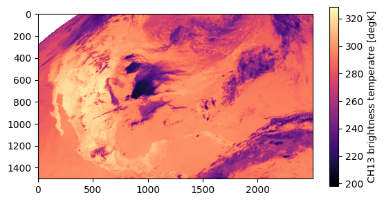
Look at the data

Let’s take a look at the CONUS 10.3-µm data.

plt.imshow(ch13, cmap='magma')
plt.colorbar(label="CH13 brightness temperatre [degK]", shrink=0.7)
plt.show()

Remap the data to MRMS projection

Great! The data look normal. But how do we transform it into a new projection? We use pyresample. There are two ways of handling this. We can use an AreaDefinition object, or a GridDefinition object. If you have the latitudes and longitudes at every point, then GridDefinition is probably easiest.

GridDefinition method

This is how you convert the satellite’s projection coordinates to latitudes and longitudes. See here for geos parameters. x and y are the “projection coordinates.” perspective_point_height is the height of the satellite above the surface of the Earth (in meters), and longitude_of_projection_origin is the longitude that the satellite is at.

sat_height = ds.goes_imager_projection.perspective_point_height
sat_longitude = ds.goes_imager_projection.longitude_of_projection_origin
x = ds['x'].data * sat_height
y = ds['y'].data * sat_height

xx,yy = np.meshgrid(x,y)

projection = pyproj.Proj(f'+proj=geos +lon_0={sat_longitude} +h={sat_height}')

lons, lats = projection(xx, yy, inverse=True)

Now let’s see how the lats and lons look.

fig, ax = plt.subplots(nrows=1, ncols=2, figsize=(10,5))
im1 = ax[0].imshow(lats)
fig.colorbar(im1, label='Latitudes [degrees]', shrink=0.5)
im2 = ax[1].imshow(lons)
fig.colorbar(im2,label='Longitudes [degrees]', shrink=0.5)
plt.show()

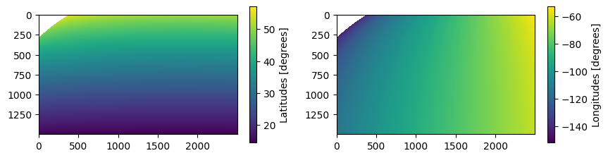
The coordinates look good to me. Now make the GridDefinition for the original projection.

goes_def = pyresample.geometry.GridDefinition(lats=lats, lons=lons)

Now we need the GridDefinition of the new projection. We are remapping to the MRMS projection. I happen to know that the projection of MRMS is “cylindrical equidistant” or “equal-lat-lon.”

• The Northwest corner point is (55, -130)

• There are 3500 latitudes and 7000 longitudes

• The resolution is 0.01 degree (approximately 1-km).

Let’s make the MRMS lats and lons and the MRMS GridDefinition. But instead of using 0.01-degree resolution, we can use 0.02-degree resolution, because the IR data is at about 2-km.

tmp_lats = np.arange(55, 20, -0.02)
tmp_lons = np.arange(-130, -60, 0.02)
mrms_lons, mrms_lats = np.meshgrid(tmp_lons, tmp_lats)
mrms_def = pyresample.geometry.GridDefinition(lats=mrms_lats, lons=mrms_lons)

Now for the actual regridding / resampling!

We will be using resample_nearest, which uses nearest-neighbor to resample. You could also use resample_gauss if you want to weight nearby pixels.

radius_of_influence is in meters. Basically, how far around the point do you want the resampling algorithm to “look”.

fill_value is the value to fill pixels where it couldn’t resample (i.e., where original data is not in the new grid definition).

Remember that this should go much faster on a half-way decent server. On Colab, it takes 15-20 seconds.

remapped_goes = pyresample.kd_tree.resample_nearest(goes_def, ch13, mrms_def, radius_of_influence=4000, fill_value=0)

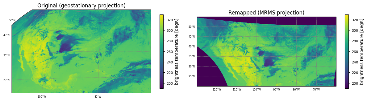
Finally, let’s plot our old data and our new data in a georeferenced format, using cartopy.

import cartopy.crs as ccrs

fig = plt.figure(figsize=(12, 6))

# Plot the unremapped data

crs = ccrs.Geostationary(central_longitude=sat_longitude)
extent = [x.min(), x.max(), y.min(), y.max()]
ax1 = fig.add_axes([0, 0, 0.47, 1], projection=crs)

orig = ax1.imshow(ch13, vmin=190, vmax=330, extent=extent, transform=crs)

gl = ax1.gridlines(
  crs=ccrs.PlateCarree(),
  draw_labels=True,
  linewidth=0.5,
  color="gray",
  linestyle="--",
)
# Customize the gridline labels
gl.top_labels = None
gl.right_labels = None
gl.xlabel_style = {"size": 6}
gl.ylabel_style = {"size": 6}

cbar1 = fig.colorbar(orig,label='brightness temperature [degK]', shrink=0.4)
cbar1.ax.tick_params(labelsize=8)
ax1.set_title("Original (geostationary projection)")


# Plot the remaped data

crs_mrms = ccrs.PlateCarree()
extent = [-130, -60, 20, 55]
ax2 = fig.add_axes([0.50, 0, 0.47, 1], projection=crs_mrms)

remapped = ax2.imshow(remapped_goes, vmin=190, vmax=330, extent=extent, transform=crs_mrms)

gl2 = ax2.gridlines(
  crs=ccrs.PlateCarree(),
  draw_labels=True,
  linewidth=0.5,
  color="gray",
  linestyle="--",
)
# Customize the gridline labels
gl2.top_labels = None
gl2.right_labels = None
gl2.xlabel_style = {"size": 6}
gl2.ylabel_style = {"size": 6}

cbar2 = fig.colorbar(remapped,label='brightness temperature [degK]', shrink=0.4)
cbar2.ax.tick_params(labelsize=8)
ax2.set_title("Remapped (MRMS projection)")


plt.show()

AreaDefinition method

The AreaDefinition method is very similar, but doesn’t require the latitudes and longitudes. In only requires knowing the extent. Let’s set up the AreaDefinition for the original and target projections. We could still use the GridDefinition for the MRMS projection if we wanted to. You can remap between AreaDefinitions and GridDefinitions interchangeably.

Note that the conversion of x and y by multipliying by sat_height still applies for the original projection.

ny, nx = ch13.shape

# Note that `area_extent` has the format: (lower_left_x, lower_left_y, upper_right_x, upper_right_y),
# which is different from the `extent` in `imshow` (lower_left_x, upper_right_x, lower_left_y, upper_right_y)

orig = pyresample.geometry.AreaDefinition('origProj', 'geosProj', 'projID1',
                                          ccrs.Geostationary(central_longitude=sat_longitude),
                                          width=nx,
                                          height=ny,
                                          area_extent=[x.min(), y.min(), x.max(), y.max()])

target = pyresample.geometry.AreaDefinition('foo', 'foo2', 'foo3',
                                          ccrs.PlateCarree(),
                                          width=len(tmp_lons),
                                          height=len(tmp_lats),
                                          area_extent=[-130, 20, -60, 55])

Remap the data. We could instead replace target with mrms_def from above.

remapped_goes_2 = pyresample.kd_tree.resample_nearest(orig, ch13, target, radius_of_influence=4000, fill_value=0)

And plot our original and remapped data.

import cartopy.crs as ccrs

fig = plt.figure(figsize=(12, 6))

# Plot the unremapped data

crs = ccrs.Geostationary(central_longitude=sat_longitude)
extent = [x.min(), x.max(), y.min(), y.max()]
ax1 = fig.add_axes([0, 0, 0.47, 1], projection=crs)

orig = ax1.imshow(ch13, vmin=190, vmax=330, extent=extent, transform=crs)

gl = ax1.gridlines(
  crs=ccrs.PlateCarree(),
  draw_labels=True,
  linewidth=0.5,
  color="gray",
  linestyle="--",
)
# Customize the gridline labels
gl.top_labels = None
gl.right_labels = None
gl.xlabel_style = {"size": 6}
gl.ylabel_style = {"size": 6}

cbar1 = fig.colorbar(orig,label='brightness temperature [degK]', shrink=0.4)
cbar1.ax.tick_params(labelsize=8)
ax1.set_title("Original (geostationary projection)")


# Plot the remaped data

crs_mrms = ccrs.PlateCarree()
extent = [-130, -60, 20, 55]
ax2 = fig.add_axes([0.50, 0, 0.47, 1], projection=crs_mrms)

remapped = ax2.imshow(remapped_goes_2, vmin=190, vmax=330, extent=extent, transform=crs_mrms)

gl2 = ax2.gridlines(
  crs=ccrs.PlateCarree(),
  draw_labels=True,
  linewidth=0.5,
  color="gray",
  linestyle="--",
)
# Customize the gridline labels
gl2.top_labels = None
gl2.right_labels = None
gl2.xlabel_style = {"size": 6}
gl2.ylabel_style = {"size": 6}

cbar2 = fig.colorbar(remapped,label='brightness temperature [degK]', shrink=0.4)
cbar2.ax.tick_params(labelsize=8)
ax2.set_title("Remapped (MRMS projection)")


plt.show()

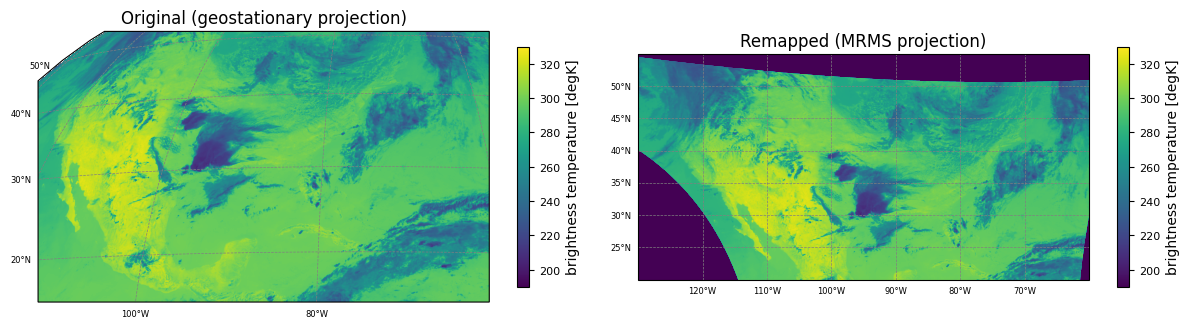
The image from the cell above should match the cell from the GridDefinition method.

Writing a WDSS2-compatible netCDF4

WDSS2 (www.wdssii.org) has some special requirements for its version of netCDF4 format:

• Data must be in equal-lat equal-lon projection.

• This means LatGridSpacing and LonGridSpacing must be constants

• There can only be one variable in each netCDF.

• Required global attributes:

• TypeName (should be the name of the variable)

• DataType (usually LatLonGrid, if not using radar)

• LatGridSpacing

• LonGridSpacing

• Latitude (NW latitude)

• Longitude (NW longitdue)

• Height

• Time (seconds since 1970-01-01 00:00:00 UTC)

• FractionalTime (not sure if this is explicitly required)

• MissingData (again, not sure if it’s required, but it’s a good idea to include)

write_netcdf function

Let’s write our remapped data in WDSS2 format. We’ll use this write_netcdf function. Read the docstring for help.

import os
import netCDF4

def write_netcdf(output_file,
                 datasets,
                 dims,
                 atts={}):

  '''
  Parameters:
  -------------
  -  output_file (str): Full path to output filename
  -  datasets (dict): Nested set of dictionaries with top-level keys as variable names.
     -  structure:
        datasets[varname1] = {'data': numpy_ndarray_object,
                              'atts':{attname1: val1,   # these are variable attributes
                                      attname2: val2
                                     },
                              'dims': (dimYName, dimXName)}.    # the dimensions of datasets[varname1]['data']
  - dims (dict): Dictionary with string keys / integer values for the dimensions of every variable written to netCDF
  - atts (dict): Dictionary for global attributes

  Returns:
  -------------
  True if successful
  '''

  print('Process started')

  os.makedirs(os.path.dirname(output_file), exist_ok=True)
  ncfile = netCDF4.Dataset(output_file,'w') #,format='NETCDF3_CLASSIC')

  #dimensions
  for dim in dims:
    ncfile.createDimension(dim,dims[dim])
  #variables

  for varname in datasets:
    if(isinstance(datasets[varname]['data'],np.ndarray)):
      dtype = str((datasets[varname]['data']).dtype)
    elif(isinstance(datasets[varname]['data'],int) or isinstance(datasets[varname]['data'],np.int32) or isinstance(datasets[varname]['data'],np.int16)):
      dtype = 'i'
    elif(isinstance(datasets[varname]['data'],float) or isinstance(datasets[varname]['data'],np.float32) or isinstance(datasets[varname]['data'],np.float16)):
      dtype = 'f'

    if('_FillValue' in datasets[varname]['atts']):
      dat = ncfile.createVariable(varname,dtype,datasets[varname]['dims'],fill_value=datasets[varname]['atts']['_FillValue'])
    else:
      dat = ncfile.createVariable(varname,dtype,datasets[varname]['dims'])
    dat[:] = datasets[varname]['data']
    #variable attributes
    if('atts' in datasets[varname]):
      for att in datasets[varname]['atts']:
        if(att != '_FillValue'): dat.__setattr__(att,datasets[varname]['atts'][att]) #_FillValue is made in 'createVariable'
  #global attributes
  for key in atts:
    ncfile.__setattr__(key,atts[key])
  ncfile.close()
  print(f'Wrote out {output_file}')


  print('Process ended')

  return True

Dataset, Dims, and atts

Now let’s create/organize our input parameters. You can add addtional attributes if you would like. Also, please note that additional global attributes may be required to view in the WDSS2 GUI, wg, but I am not sure.

import collections

# Get timestamp
epoch_seconds = int((abidt - datetime.datetime(1970,1,1,0,0)).total_seconds())

remapped_ny, remapped_nx = remapped_goes.shape

dims = collections.OrderedDict()
dims['Lat'] = remapped_ny
dims['Lon'] = remapped_nx

varname = 'remapped_goes'
dataset = {varname:{'data':remapped_goes,
                    'dims':('Lat','Lon'),
                    'atts':{'units':'degK',
                            'missing_data': 0}}}
atts = collections.OrderedDict()
atts['TypeName'] = varname
atts['DataType'] = 'LatLonGrid'
atts['LatGridSpacing'] = 0.02   # we created the MRMS projection at 0.02-degree resolution
atts['LonGridSpacing'] = 0.02   # we created the MRMS projection at 0.02-degree resolution
atts['Latitude'] = 55
atts['Longitude'] = -130
atts['Height'] = 0.             # I believe this is usually ignored unless you are dealing with tilts
atts['Time'] = epoch_seconds
atts['FractionalTime'] = 0.
atts['MissingData'] = 0
atts['attributes'] = ""

Write out the netCDF

And write the netCDF. The name of the netCDF must be a timestamp, in format: '%Y%m%d-%H%M%S.netcdf', and it should be in a directory that is named varname.

outnc = abidt.strftime(f'outnc/{varname}/%Y%m%d-%H%M%S.netcdf')

write_netcdf(outnc, dataset, dims, atts=atts)

Process started
Wrote out outnc/remapped_goes/20240528-180100.netcdf
Process ended

True

Inspect the output

Now let’s look at the netCDF.

nc = netCDF4.Dataset('outnc/remapped_goes/20240528-180100.netcdf')
print(nc)
data = nc.variables['remapped_goes'][:]
nc.close()

crs_mrms = ccrs.PlateCarree()
extent = [-130, -60, 20, 55]

fig = plt.figure(figsize=(12, 8))

ax = fig.add_axes([0.50, 0, 0.47, 1], projection=crs_mrms)

remapped = ax.imshow(data, vmin=190, vmax=330, extent=extent, transform=crs_mrms)

gl = ax.gridlines(
  crs=ccrs.PlateCarree(),
  draw_labels=True,
  linewidth=0.5,
  color="gray",
  linestyle="--",
)
# Customize the gridline labels
gl.top_labels = None
gl.right_labels = None
gl.xlabel_style = {"size": 6}
gl.ylabel_style = {"size": 6}

cbar = fig.colorbar(remapped,label='brightness temperature [degK]', shrink=0.4)
cbar.ax.tick_params(labelsize=8)
ax.set_title("Remapped GOES (from netCDF)")

plt.show()

<class 'netCDF4._netCDF4.Dataset'>
root group (NETCDF4 data model, file format HDF5):
    TypeName: remapped_goes
    DataType: LatLonGrid
    LatGridSpacing: 0.02
    LonGridSpacing: 0.02
    Latitude: 55
    Longitude: -130
    Height: 0.0
    Time: 1716919260
    FractionalTime: 0.0
    MissingData: 0
    attributes:
    dimensions(sizes): Lat(1750), Lon(3500)
    variables(dimensions): float32 remapped_goes(Lat, Lon)
    groups:

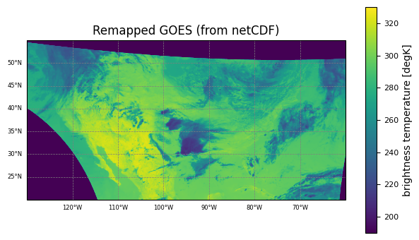
Looks good to me! This netCDF should now work in WDSS2 algorithms such as w2segmotionll, w2cropconv, etc.